A streamlined guide using the SimulationStudy manager.
Use the SimulationStudy manager to handle the entire lifecycle: storage, diagnostics, active refinement, analysis, and intelligent caching.
Note
In this tutorial, we will intentionally feed the study “bad” data (with a large gap in the input space) to demonstrate how the active learning module automatically identifies and fixes issues. We will also demonstrate how the new Layered Caching engine makes exploring multi-dimensional parameter spaces nearly instantaneous.
1. Setup, Generation & Smart Initialization
We’ll define a simulated physics function with heteroscedastic noise and generate an initial design containing a deliberate gap between 3mm and 7mm.
Notice that we no longer need to explicitly define our input columns when creating the SimulationStudy; the manager will automatically infer them from the data!
import numpy as npimport pandas as pdimport timefrom digiqual import SimulationStudy# --- Define the Physics ---def apply_physics(df):"""Simulates a signal with quadratic trends and heteroscedastic noise.""" signal = (10.0+ (2.0* df["Length"])+ (0.5* df["Length"] **2)- (0.1* np.abs(df["Angle"])) ) noise_scale =0.5+ (1.5* df["Roughness"]) noise = np.random.normal(loc=0, scale=noise_scale, size=len(df))return signal + noise# --- Create Flawed Data (Gap between 3mm and 7mm) ---df1 = pd.DataFrame( {"Length": np.random.uniform(0.1, 3.0, 40),"Angle": np.random.uniform(-10, 10, 40),"Roughness": np.random.uniform(0, 0.5, 40), })df2 = pd.DataFrame( {"Length": np.random.uniform(7.0, 10.0, 40),"Angle": np.random.uniform(-10, 10, 40),"Roughness": np.random.uniform(0, 0.5, 40), })df_initial = pd.concat([df1, df2], ignore_index=True)df_initial["Signal"] = apply_physics(df_initial)# --- The NEW Smarter Initialization ---# 1. Initialize with a clean slatestudy = SimulationStudy()# 2. Add data: It automatically infers 'Length', 'Angle', 'Roughness' as inputs!study.add_data(df_initial, outcome_col="Signal", overwrite=True)# Test the UI Helper methodsprint(f"Inferred Inputs: {study.inputs}")threshold_defaults = study.get_data_summary("Signal")print(f"Auto-Threshold suggestion (Median Signal): {threshold_defaults['median']:.2f}")
Data initialized/overwritten. Total rows: 80
Inferred Inputs: ['Length', 'Angle', 'Roughness']
Auto-Threshold suggestion (Median Signal): 34.35
TipNote on Design Generation: generate_lhs
When creating initial space-filling designs programmatically (instead of synthetic random samples), you can use the digiqual.sampling.generate_lhs(n, ranges) utility. The library automatically applies a greedy max-min distance reordering algorithm to the generated coordinates. This ensures that any prefix of size \(k\) is as space-filling as possible, allowing you to stop the physical solver early or execute runs incrementally while maintaining optimal coverage of the parameter space.
2. Diagnosis (Detecting the Issue)
We ask the SimulationStudy manager to diagnose the health of our experiment.
Warning
Because of our deliberate gap, we expect the diagnostic engine to flag the Input Coverage test as failed.
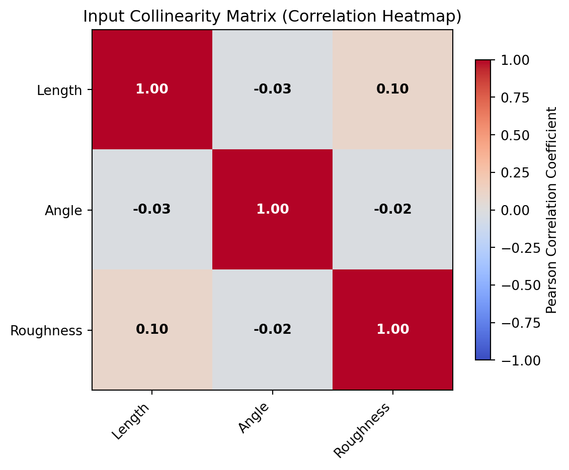
Additionally, the diagnostic suite now automatically checks for multicollinearity by calculating the Variance Inflation Factor (VIF) for each input variable (controlled by the max_allowed_vif parameter, which defaults to 5.0).
You can also visually inspect collinearity using the plot_collinearity() method, which renders a correlation matrix heatmap with VIF and correlation coefficient annotations.
study.plot_collinearity()
Figure 1: Collinearity analysis matrix
3. Adaptive Refinement (The Fix)
Instead of manually guessing where to add new simulations, we use the refine() method.
Detect: It automatically targets the exact region where the gap or uncertainty exists.
Generate: It outputs a dataframe of new input coordinates.
Execute & Store: Appending the results back using add_data() automatically clears the mathematical caches to ensure your next analysis uses the updated physics!
# Generate active learning samples (20 points to fill the gap)new_samples = study.refine(n_points=20)ifnot new_samples.empty:# Apply the exact same physics model to the new points new_samples["Signal"] = apply_physics(new_samples)# Add back to study (This strips metadata and drops the caches!) study.add_data(new_samples)# Re-run diagnostics to confirm the green lightstudy.diagnose()
Diagnostics flagged issues. Initiating Active Learning...
 -> Strategy: Exploration (Filling gaps in Length)
Data appended. Total rows: 100
Running validation...
Validation passed. 100 valid rows ready.
Checking sample sufficiency...
Test
Variable
Metric
Value
Threshold
Pass
0
Input Coverage
Length
Max Gap Ratio
0.0523
< 0.20
True
1
Input Coverage
Angle
Max Gap Ratio
0.0415
< 0.20
True
2
Input Coverage
Roughness
Max Gap Ratio
0.0460
< 0.20
True
3
Model Fit (CV)
Signal
Mean R2 Score
0.9977
> 0.50
True
4
Bootstrap Convergence
Signal
Avg CV (Rel Std Dev)
0.0105
< 0.15
True
5
Bootstrap Convergence
Signal
Max CV (Rel Std Dev)
0.0185
< 0.30
True
6
Collinearity Check
Length
VIF
1.0849
< 5.00
True
7
Collinearity Check
Angle
VIF
1.0077
< 5.00
True
8
Collinearity Check
Roughness
VIF
1.0929
< 5.00
True
4. Reliability Analysis & Layered Caching
With a validated dataset, we can now run the complete PoD pipeline.
Tip
The SimulationStudy engine uses a Layered Caching Architecture.
When you run .pod() for the first time, it evaluates all possible models and stores the mathematical heavy-lifting in memory. If you want to change a parameter slice (e.g., investigating a different ‘Angle’), you can use .update_slice() to instantly generate a new PoD curve without refitting the model!
The single pod() method automatically handles:
Monte-Carlo Integration (marginalising out Nuisance variables using Uniform or custom distributions like Normal, Lognormal, and Weibull)
Distribution Inference (finding the best error distribution)
Bootstrapping (generating confidence bounds)
NoteWhy Configure Custom Nuisance Profiles?
In the code snippet below, we pass nuisance_dists={"Roughness": ("norm", (0.25, 0.08))} to the .pod() engine instead of letting it default to a Uniform distribution.
If we assume surface roughness is Uniformly distributed between its extreme bounds, the Monte Carlo integration treats an incredibly rough, worst-case surface as just as likely to occur as a nominal, well-machined surface. This would unnecessarily degrade our final Probability of Detection curve. By specifying a Normal distribution centered around the nominal design specification (\(0.25\) with a standard deviation of \(0.08\)), digiqual samples coordinates that mirror real-world production distributions. This ensures your final calculated reliability curves represent field performance, rather than an unphysical worst-case scenario.
# --- RUN 1: Baseline Analysis ---# Expect this to take a moment as it trains models# and optimizes variance bandwidth.# We configure 'Roughness' with a custom Normal distribution: mean=0.25, std=0.08t0 = time.time()results = study.pod( poi_col="Length", nuisance_col=["Roughness"], # Integrate over roughness slice_values={"Angle": 0.0}, # Hold Angle strictly at 0.0! threshold=34.0, n_boot=0, # Skipping bootstrap for the speed demonstration nuisance_dists={"Roughness": ("norm", (0.25, 0.08))},)print(f"Run 1 completed in: {time.time() - t0:.4f} seconds")# Access the calculated Sobol sensitivity indices for each input parameterprint("Sobol Sensitivity Indices (Total Effect):")for var, val in results["sobol_indices"].items():print(f" {var}: {val *100:.1f}%")# --- RUN 2: Interactive Slicing ---# Changing the constant 'Angle' slice triggers# a Cache Hit for the model and variance!t1 = time.time()new_results = study.update_slice({"Angle": 5.0})print(f"Run 2 completed in: {time.time() - t1:.4f} seconds (Near Instant!)")print(f"New a90/95 point at Angle 5.0: {new_results['a90_95']:.3f}")
--- Starting Reliability Analysis (PoIs: ['Length'] - Nuisance: ['Roughness']) ---
-> Slicing surface at: {'Angle': 0.0}
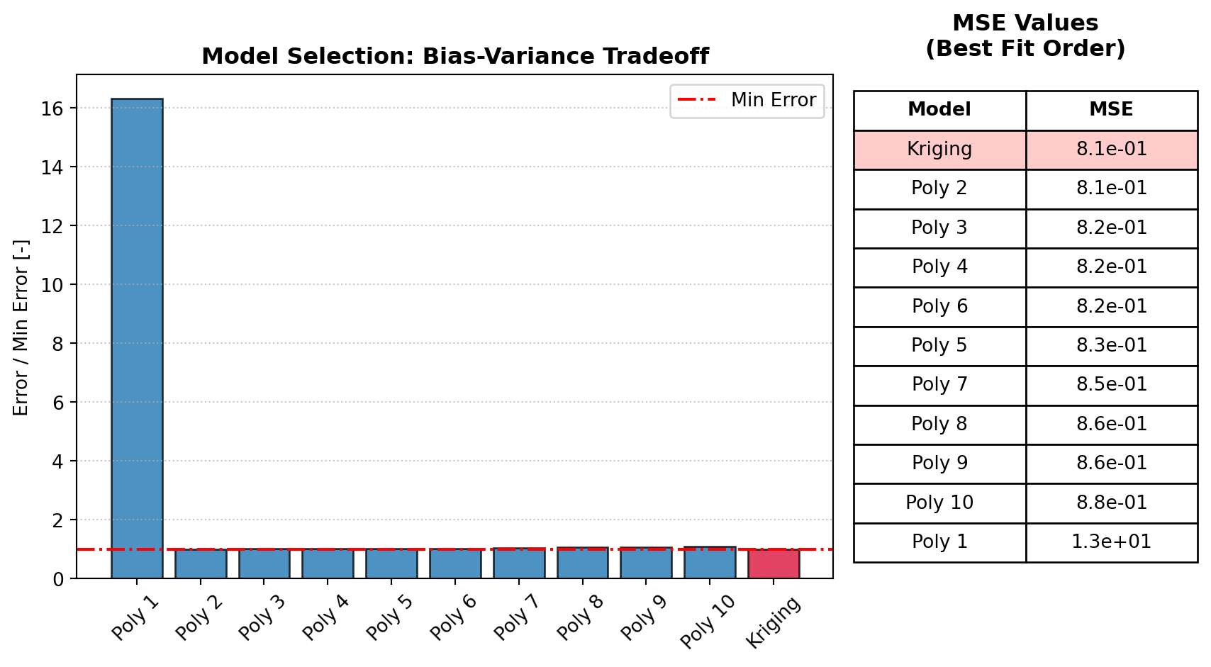
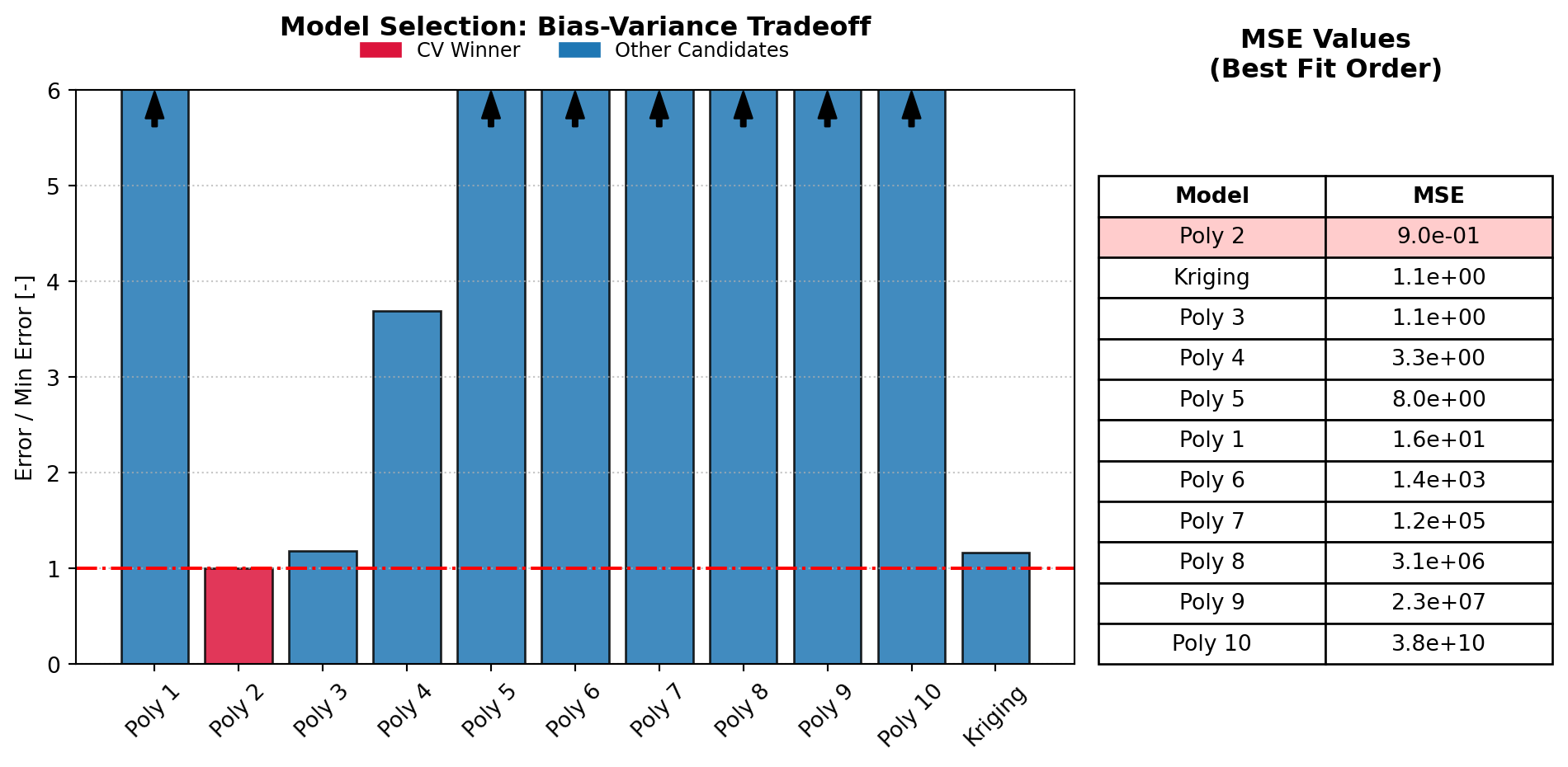
1. Training all surrogate models (Cache Miss)...
-> Selected Model: Polynomial (Degree 3)
2. Fitting Variance Model & Inferring Distribution (Cache Miss)...
-> Optimizing bandwidth via LOO-CV...
-> Calculating Total-Order Sobol Indices...
-> Smoothing Bandwidth: 2.3218
-> Selected Distribution: norm
3. Integrating PoD Curve from Scratch (Cache Miss)...
4. Skipping Bootstrap (n_boot=0)...
--- Analysis Complete ---
Run 1 completed in: 0.9520 seconds
Sobol Sensitivity Indices (Total Effect):
Length: 100.0%
Angle: 0.0%
Roughness: 0.0%
--- Starting Reliability Analysis (PoIs: ['Length'] - Nuisance: ['Roughness']) ---
-> Slicing surface at: {'Angle': 5.0}
1. Loading surrogate models from cache (Cache Hit)...
-> Selected Model: Polynomial (Degree 3)
2. Loading Variance Model, Distribution & Sobol from cache (Cache Hit)...
-> Smoothing Bandwidth: 2.3218
-> Selected Distribution: norm
3. Integrating PoD Curve from Scratch (Cache Miss)...
4. Skipping Bootstrap (n_boot=0)...
--- Analysis Complete ---
Run 2 completed in: 0.2367 seconds (Near Instant!)
New a90/95 point at Angle 5.0: nan
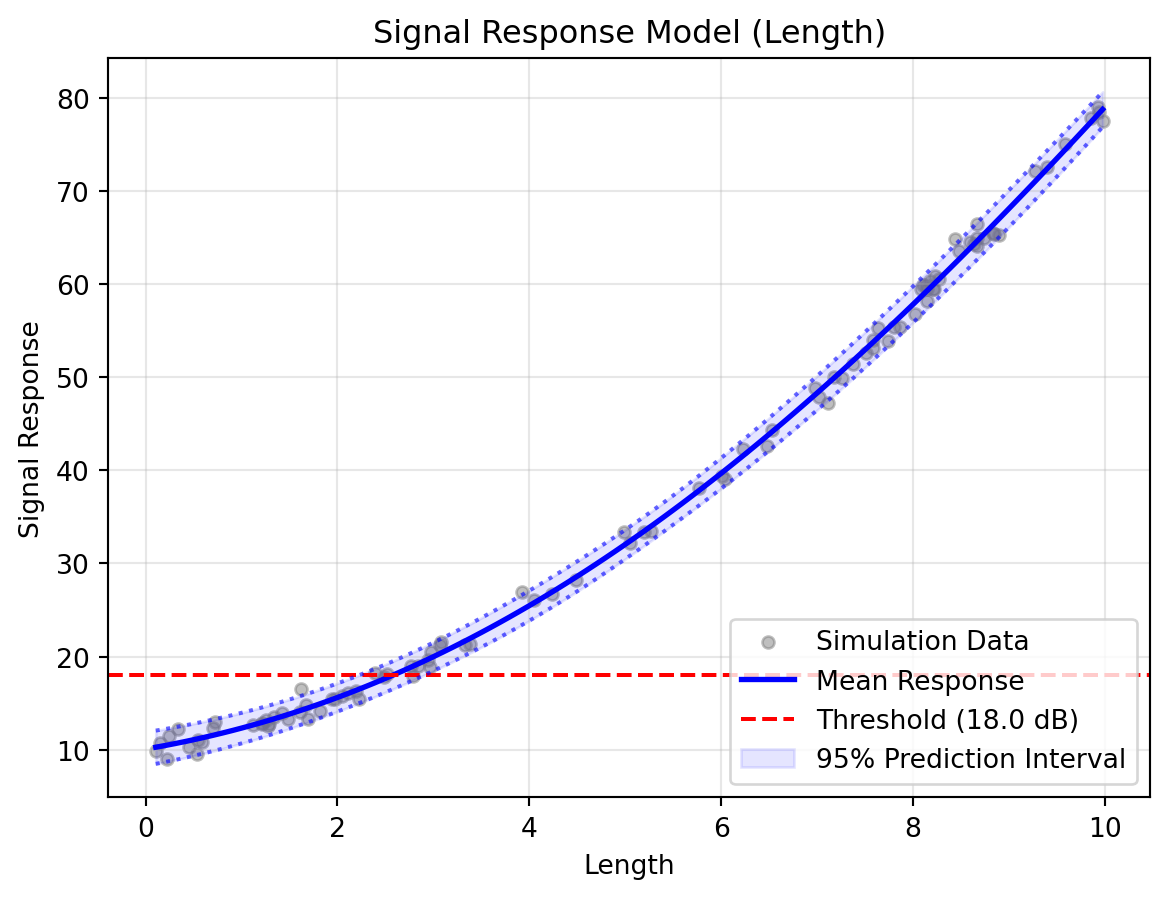
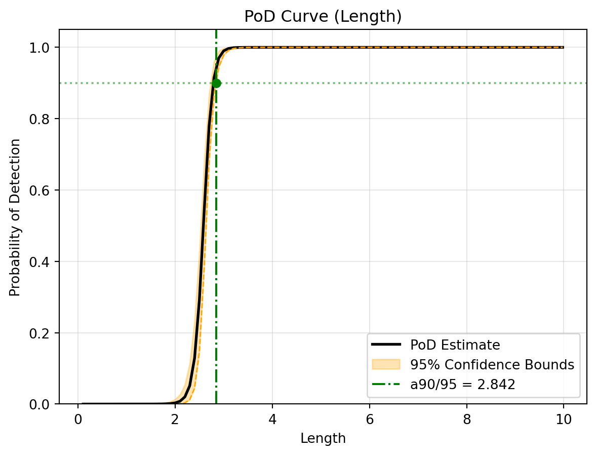
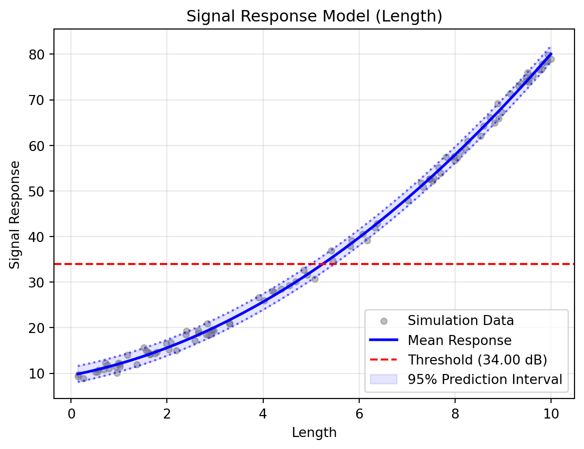
# Visualise the results of the final active slicestudy.visualise()
To calculate reliability indices with confidence intervals, we run the bootstrapping algorithm.
Unlike traditional tools that compute only a single confidence interval (e.g., 95%), digiqual runs bootstrapping once to extract bounds for multiple confidence levels (50%, 90%, 95%, 99%) across standard target PoDs (50%, 90%, 95%, 99%) simultaneously.
These are saved in the results dictionaries:
results['ci_bounds']: Maps confidence levels to lower/upper curves.
results['reliability_table']: Maps (target_pod_percent, confidence_level) tuples to their corresponding flaw sizing reliability indices (e.g., a90/95).
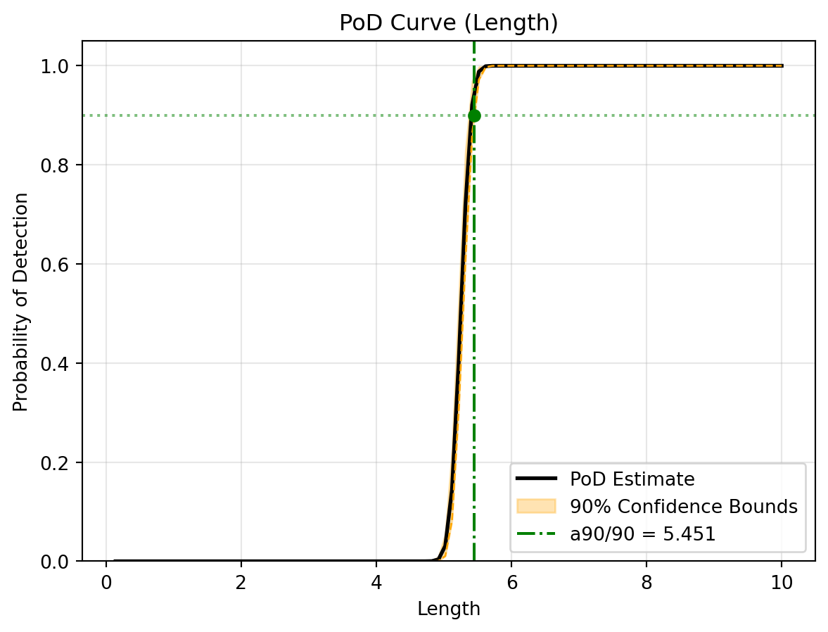
# Run the parallelised bootstrap to get multi-level confidence boundst2 = time.time()uq_results = study.pod( poi_col="Length", nuisance_col=["Roughness"], slice_values={"Angle": 5.0}, threshold=34.0, n_boot=100, # Small value for quick demonstration n_jobs=-1# Use all available CPU cores)print(f"UQ Bootstrapping completed in: {time.time() - t2:.4f} seconds")# Access the custom reliability matrix values# Print the calculated a90/95 and a90/90 valuesa90_95 = uq_results["reliability_table"].get((90, 95))a90_90 = uq_results["reliability_table"].get((90, 90))print(f"a90/95: {a90_95:.3f} mm")print(f"a90/90: {a90_90:.3f} mm")
(c) UQ Reliability S-curve with 90% Confidence Bounds for a 90% target PoD
Figure 3: Reliability Analysis Results
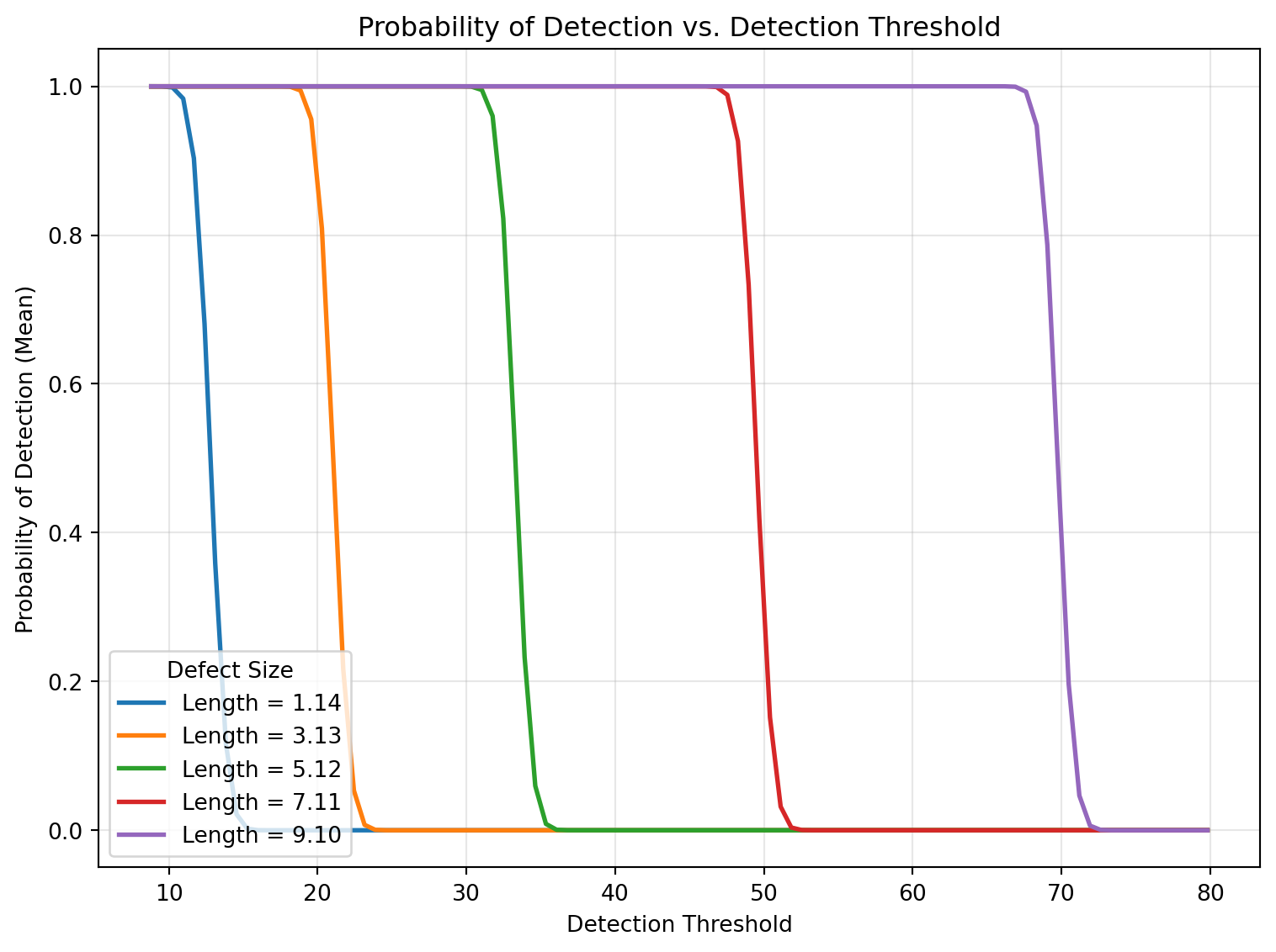
Threshold Sensitivity Plots
Using the cached 100-threshold spectrum, we can also generate a sensitivity plot using plot_pod_vs_threshold() to see how changing the threshold affects PoD across defect sizes.