Automated Optimisation

The optimise method allows you to run a complete “Active Learning” loop. DigiQual will generate an initial design, run your external solver, check the results, and automatically add new points where the model is weak.

1 The Active Learning Lifecycle

When you trigger the optimise method, DigiQual acts as an orchestrator, completing the following active learning loop until statistical requirements are satisfied.

flowchart TD
    A[1. Initialise - Generate LHS Design] --> B(2. Execute Solver)
    B --> C{3. Diagnostics}
    C -->|Healthy| D[(Final Validated Data)]
    C -->|Fails Check| E[4. Refinement - Generate Targeted Samples]
    E --> B

1.1 Breakdowns of the Steps

Initialisation: If you have no existing data, DigiQual generates an initial batch of input coordinates using a space-filling Latin Hypercube Sample (see Section 2.1).
Execution: It passes these coordinates to your solver and waits for the results.
Diagnostics (Sense): Once the results are back, DigiQual runs the diagnostic tests in Section 2.2: input coverage gaps, model fit, bootstrap stability and multicollinearity.
Refinement (Decide & Act): If the diagnostics fail, DigiQual generates targeted new samples exactly where the model needs them most (e.g., in the middle of an empty gap, or in highly uncertain regions) and repeats the loop.

2 Sampling & Diagnostics

The same sampling and diagnostic tools are used by optimise, by study.diagnose() / study.refine() in the Quick Start, and by the Experimental Design and Simulation Diagnostics tabs of the app.

2.1 Space-filling designs

digiqual.sampling.generate_lhs(n, ranges) (the app’s Experimental Design tab) draws a Latin Hypercube Sample over the input ranges. It then reorders the points with a greedy max-min distance algorithm: each next point is the one furthest from all points chosen so far. As a result, any first \(k\) rows of the design are themselves as space-filling as possible, so you can run the simulations in order and stop early, or run them in batches, and still have good coverage.

2.2 Diagnostic tests

The diagnostics check whether the data is good enough to fit a reliable model. Each test has a threshold you can change, as an argument to diagnose() / optimise() or in the app:

Test	What it measures	Passes when (default)
Input Coverage	For each input, the largest gap between neighbouring sorted values, as a fraction of its range	gap ratio < 0.20 (`max_gap_ratio`)
Model Fit (CV)	Cross-validated \(R^2\) of a cubic polynomial: is there a learnable signal?	\(R^2\) > 0.50 (`min_r2_score`)
Bootstrap Convergence (average)	Spread (std) of bootstrap predictions of a quadratic model at the 10th, 50th and 90th percentiles of the inputs, divided by the std of the response, averaged	< 0.15 (`max_avg_cv`)
Bootstrap Convergence (worst)	The largest of those relative spreads	< 0.30 (`max_max_cv`)
Collinearity Check	Variance Inflation Factor of each input against the others	VIF ≤ 5.0 (`max_allowed_vif`)

The bootstrap spread is measured relative to the scatter of the response, so a signal recorded near zero (e.g. in dB) or with a large constant offset is judged fairly. Versions up to 0.27 divided by the mean prediction instead, which made near-zero signals fail regardless of stability.

If a test fails, refinement (study.refine(), or the app’s Remediation tool) generates targeted new points: in the largest coverage gaps, and where a bootstrap committee of models disagrees most (Query-by-Committee). Failed solver runs are excluded from future sampling (see the graveyard, below).

3 Connecting Your External Solver

To automate this process, DigiQual needs to communicate with your simulation model (whether that is a Python function, MATLAB script, or heavy FEA software like Ansys). It does this using the Executor pattern.

DigiQual provides three built-in Executors to bridge the gap:

PythonExecutor (In-Memory): Best for purely Python-based mathematical models or surrogate models. It runs entirely in memory for maximum speed.
CLIExecutor (Process Isolation): Best for heavy physics engines (FEA/CFD) or heavy Python FEA scripts. It writes the inputs to a temporary CSV and spawns a completely isolated Operating System process to solve it. This guarantees that 100% of the solver’s memory is cleared after every run, preventing memory leaks.
MatlabExecutor: A specialized wrapper that automatically handles the complex terminal syntax required to run MATLAB in a headless “batch” mode.

(See Section 5 for examples on connecting MATLAB and external software.)

3.1 Handling Failures (Graveyard)

If your external solver crashes or fails to converge for a specific input row (e.g., a meshing error), your solver should return NaN or leave the outcome blank. DigiQual will automatically detect this and add those coordinates to a “graveyard”, ensuring the active learning loop navigates around that “dead zone” and never samples that exact region again!

4 The Auto-Pilot Workflow

Let’s walk through setting up a complete optimisation loop using a pure Python model.

4.1 Define a Solver and Executor

For this tutorial, we will write a standard Python function to simulate our physics. We will then wrap it in the PythonExecutor.

import numpy as np
from digiqual.executors import PythonExecutor


def mock_sensor_model(row):
    """A simulated physics model with noise."""
    length = row["Length"]
    angle = row["Angle"]
    roughness = row["Roughness"]

    # 1. THE DEAD ZONE (Trigger Graveyard Tracking)
    if 4.0 < length < 6.0 and abs(angle) > 30:
        return np.nan

    # 2. BASE SIGNAL (Cubic Trend + Interaction + Attenuation)
    # Roughness absorbs and scatters the signal, lowering the mean response.
    base_signal = (
        5.0
        + (5.0 * length)
        - (0.8 * (length**2))
        + (0.1 * (length**3))
        + (angle * 0.1)
        - (0.05 * length * abs(angle))
        - (roughness * 5.0)  # <--- Roughness penalty
    )

    # 3. HETEROSCEDASTIC, NON-NORMAL NOISE
    # Roughness also makes the signal noisier and harder to read.
    noise_scale = 0.5 + (length * 0.4) + (roughness * 1.0)

    noise = np.random.gumbel(loc=0, scale=noise_scale)
    noise -= noise_scale * 0.57721

    signal = base_signal + noise

    return signal


# Wrap our function in the Executor
executor = PythonExecutor(solver_func=mock_sensor_model, outcome_col="Signal")

4.2 Configure the Study

We define our input variables and the ranges we want to explore.

from digiqual.core import SimulationStudy

# Define inputs ranges
ranges = {"Length": (0.0, 10.0), "Angle": (-45.0, 45.0), "Roughness": (0, 1)}

# Initialise
study = SimulationStudy()

4.3 Run Optimisation

This single command handles the entire Active Learning loop:

study.optimise(
    executor=executor,
    ranges=ranges,
    n_start=20,  # Initial batch size
    n_step=10,  # Refinement batch size
    max_iter=5,  # Safety limit for the loops
    max_hours=1.5,  # Time limit to safely stop after 1.5 hours
    outcome_col="Signal"
)


========================================
      STARTING ADAPTIVE OPTIMIZATION
========================================
--- Iteration 0: Generating Initial Design (20 points) ---
   -> Executing Python model for 20 points...

--- Iteration 1: Diagnostics Check ---
>> Model invalid. Refining design...
Diagnostics flagged issues. Initiating Active Learning...
 -> Active Graveyard Tracker: Protecting against 2 known bad regions.
 -> Strategy: Exploitation (Targeting high uncertainty regions)
--- Running Batch 1 (10 points) ---
   -> Executing Python model for 10 points...

--- Iteration 2: Diagnostics Check ---
>> Model invalid. Refining design...
Diagnostics flagged issues. Initiating Active Learning...
 -> Active Graveyard Tracker: Protecting against 2 known bad regions.
 -> Strategy: Exploitation (Targeting high uncertainty regions)
--- Running Batch 2 (10 points) ---
   -> Executing Python model for 10 points...

--- Iteration 3: Diagnostics Check ---
>> Model invalid. Refining design...
Diagnostics flagged issues. Initiating Active Learning...
 -> Active Graveyard Tracker: Protecting against 3 known bad regions.
 -> Strategy: Exploitation (Targeting high uncertainty regions)
--- Running Batch 3 (10 points) ---
   -> Executing Python model for 10 points...

--- Iteration 4: Diagnostics Check ---
>> Model invalid. Refining design...
Diagnostics flagged issues. Initiating Active Learning...
 -> Active Graveyard Tracker: Protecting against 6 known bad regions.
 -> Strategy: Exploitation (Targeting high uncertainty regions)
--- Running Batch 4 (10 points) ---
   -> Executing Python model for 10 points...

--- Iteration 5: Diagnostics Check ---
>> Model invalid. Refining design...
Diagnostics flagged issues. Initiating Active Learning...
 -> Active Graveyard Tracker: Protecting against 6 known bad regions.
 -> Strategy: Exploitation (Targeting high uncertainty regions)
--- Running Batch 5 (10 points) ---
   -> Executing Python model for 10 points...

----------------------------------------
>>> SEARCH COMPLETE <<<
Total Time:      0.01 minutes
Successful Runs: 64
Failed Runs:     6 (in graveyard)
Total Attempted: 70
----------------------------------------

Data initialized/overwritten. Total rows: 64

4.4 View Results

Once the loop finishes, study.data contains all the valid simulation results accumulated across all refinement iterations.

print(f"Total Simulations Run: {len(study.data)}")

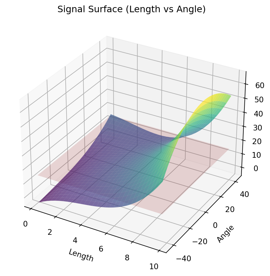
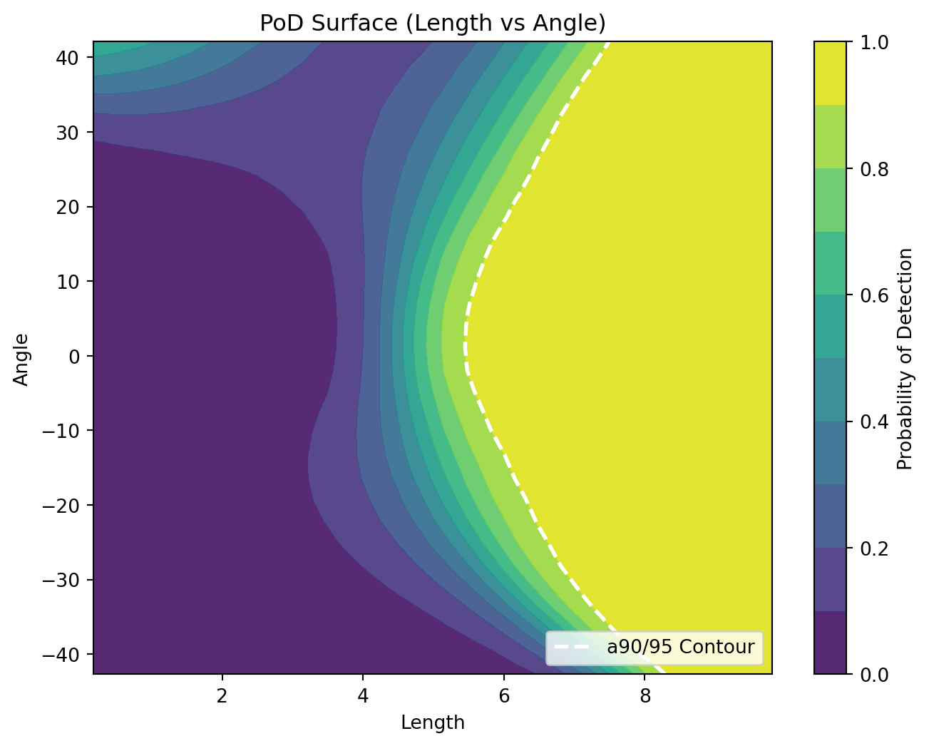
# We can evaluate the PoD mapping out the Nuisance Angle!
_ = study.pod(
    poi_col=["Length", "Angle"], nuisance_col="Roughness", threshold=15, n_jobs=-1
)
study.visualise()

5 Appendix: Real-World Wrapper Examples

When connecting DigiQual to external engines like MATLAB or Ansys, you will use the heavy-duty Executors.

5.1 Example A: Connecting to MATLAB

📥 Download MATLAB Executor Demo 📥 Download Dummy MATLAB Solver

The MatlabExecutor makes connecting to MATLAB effortless. You simply write a top-level MATLAB function that reads an input CSV, does the math, writes an output CSV, and exits.

5.1.1 The MATLAB Solver (`matlab_wrapper.m`)

function matlab_wrapper(input_csv, output_csv)
    df = readtable(input_csv);
    num_rows = height(df);

    % Pre-allocating with NaN is a safer default than zeros
    signal_results = NaN(num_rows, 1);

    for i = 1:num_rows
        % --- NEW: Wrap the physics calculation in a try...catch block ---
        try
            L = df.Length(i);
            theta = df.Angle(i);

            % Insert your complex MATLAB physics here
            signal_results(i) = (L^3) * 0.5 + theta;

        catch ME
            % If the simulation fails, catch the error and log it safely
            fprintf('Error on row %d: %s\n', i, ME.message);

            % Assign NaN so DigiQual knows this point failed and sends it to the graveyard
            signal_results(i) = NaN;
        end
    end

    df.Signal = signal_results;
    writetable(df, output_csv);

    exit; % CRITICAL: Exit MATLAB to hand control back to DigiQual
end

5.1.2 The DigiQual Execution

You just provide the name of the MATLAB file. The Executor builds the headless terminal command automatically.

from digiqual.executors import MatlabExecutor

executor = MatlabExecutor(wrapper_name="matlab_wrapper")
study.optimise(executor=executor, ranges=ranges, outcome_col="Signal")

5.2 Example B: Command Line Software (Ansys/Abaqus)

📥 Download CLI Executor Demo 📥 Download Dummy FEA Script

For software triggered via the command line, use the CLIExecutor. You must provide a command template containing {input} and {output} placeholders. DigiQual will write the design space to a temporary input CSV, spawn the terminal command, and read the resulting output CSV.

5.2.1 The External Solver Script (`run_ansys_simulation.py`)

This script represents your standalone software. It must accept the input and output file paths as command-line arguments, read the input CSV, perform its calculations, and save the output CSV.

import sys
import pandas as pd


def run_simulation(input_csv, output_csv):
    # 1. Read the input coordinates generated by DigiQual
    df = pd.read_csv(input_csv)

    signals = []
    # 2. Run the solver for each row
    for _, row in df.iterrows():
        length = row["Length"]
        angle = row["Angle"]

        # Insert your complex FEA/external physics here
        signal = (length**3) * 0.5 + angle
        signals.append(signal)

    # 3. Append the results and save
    df["Signal"] = signals
    df.to_csv(output_csv, index=False)


if __name__ == "__main__":
    # sys.argv[1] is the {input} path, sys.argv[2] is the {output} path
    run_simulation(sys.argv[1], sys.argv[2])

5.2.2 The DigiQual Execution

You define the exact terminal command needed to run the script above, and pass it to the CLIExecutor.

from digiqual.executors import CLIExecutor

# The exact command you would type into your terminal
cmd_template = "python run_ansys_simulation.py {input} {output}"

executor = CLIExecutor(command_template=cmd_template)
study.optimise(executor=executor, ranges=ranges, outcome_col="Signal")