Comparing Classical vs. Generalised Reliability

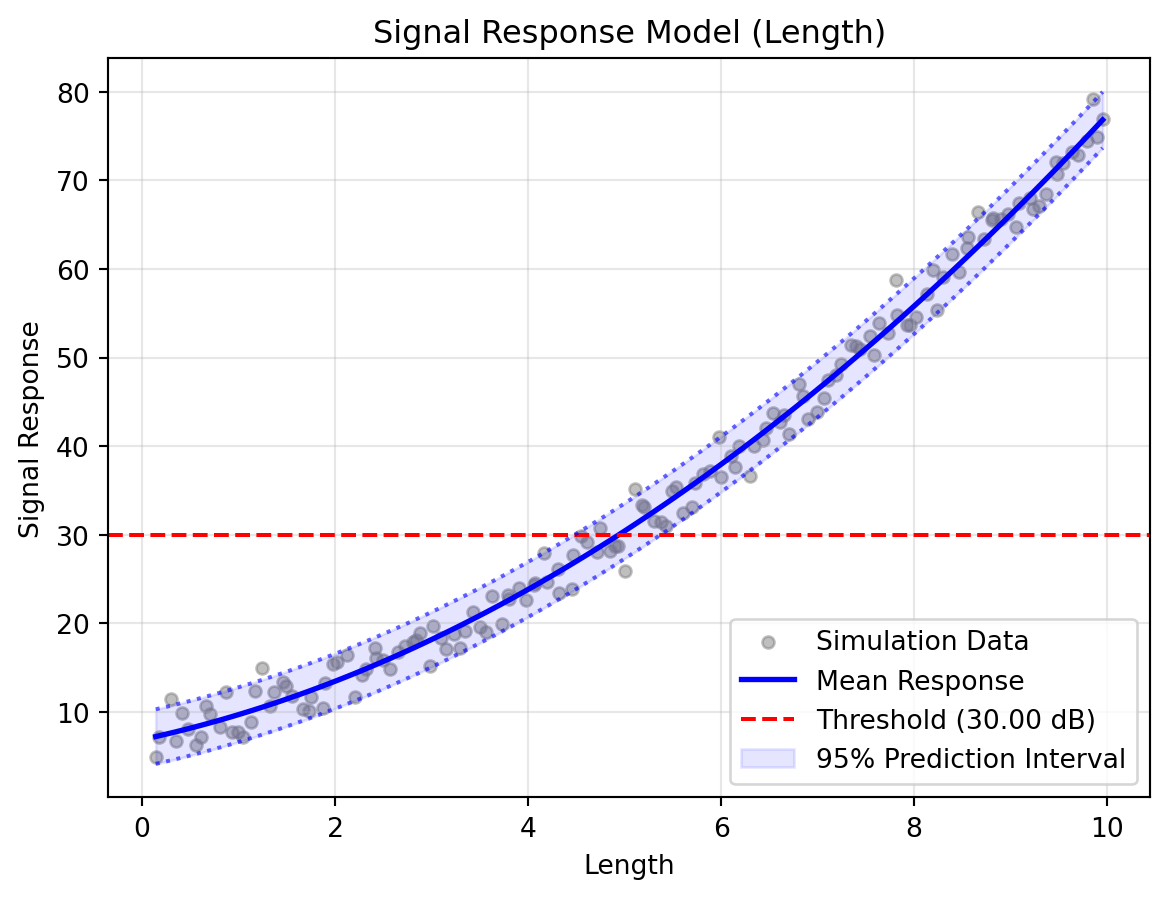
A side-by-side comparison of the linear \(\hat{a}\) versus \(a\) method and the relaxed generalised method using DigiQual.

In this tutorial, we will explore the differences between the classical linear PoD approach and the generalised active-learning approach.

The classical method assumes a strictly linear relationship and constant noise (homoskedasticity). When physical reality violates these assumptions—such as signals that curve or noise that scales with defect size—the classical method can produce misleading confidence bounds. We will generate a synthetic dataset that deliberately breaks these rules to see how both methods handle it.

1. Setup & Data Generation

First, we will simulate a physics scenario where the signal response grows quadratically and the noise increases with the flaw size.

import numpy as np
import pandas as pd
import matplotlib.pyplot as plt

from digiqual.core import SimulationStudy
from digiqual.sampling import generate_lhs


# --- Define the Non-Linear Physics ---
def apply_physics(df):
    """Simulates a multidimensional signal with nuisance parameters."""
    # Base Signal: Quadratic trend (2*L + 0.5*L^2)
    # Angle Penalty: Misalignment (-0.1*Angle) reduces signal
    signal = (
        10.0
        + (2.0 * df["Length"])
        + (0.5 * df["Length"] ** 2)
        - (0.1 * np.abs(df["Angle"]))
    )

    # Heteroscedastic Noise: Higher roughness = More scatter
    noise_scale = 0.5 + (1.5 * df["Roughness"])
    noise = np.random.normal(loc=0, scale=noise_scale, size=len(df))

    return signal + noise


# --- 2. Create the Dataset ---
# We use Latin Hypercube Sampling to efficiently cover the 3D space
vars_df = pd.DataFrame(
    [
        {"Name": "Length", "Min": 0.1, "Max": 10.0},
        {"Name": "Angle", "Min": -45.0, "Max": 45.0},
        {"Name": "Roughness", "Min": 0.0, "Max": 1.0},
    ]
)

np.random.seed(42)
df = generate_lhs(ranges=vars_df, n=150)  # 150 points for 3D space
df["Signal"] = apply_physics(df)

study = SimulationStudy()
study.add_data(df, outcome_col="Signal")

Data initialized/overwritten. Total rows: 150

2. The Classical Approach (Linear)

We will start with the traditional \(\hat{a}\) versus \(a\) method. We will apply a logarithmic transformation to the Length axis (xlog=True) to give the linear model its best chance at fitting the curved data.

Note: Instead of using the complex analytical formulas from MIL-HDBK-1823A, we are using modern bootstrapping to evaluate the confidence bounds. This strictly maintains the classical assumptions (constant variance and normal errors) while easily calculating the 95% worst-case curve.

# Run the classical linear PoD analysis
linear_results = study.linear_pod(
    poi_col="Length",
    threshold=30,
    xlog=True,
    ylog=True,
    n_jobs=-1,  # Use all CPU cores for fast bootstrapping
)

# Visualise the standard signal fit and PoD curve
study.visualise_linear(show=True)

Running validation...
Validation passed. 150 valid rows ready.
--- Starting Linear a-hat vs a Analysis (PoI: Length) ---
Running Bootstrap (1000 iterations) to establish classical confidence bounds...
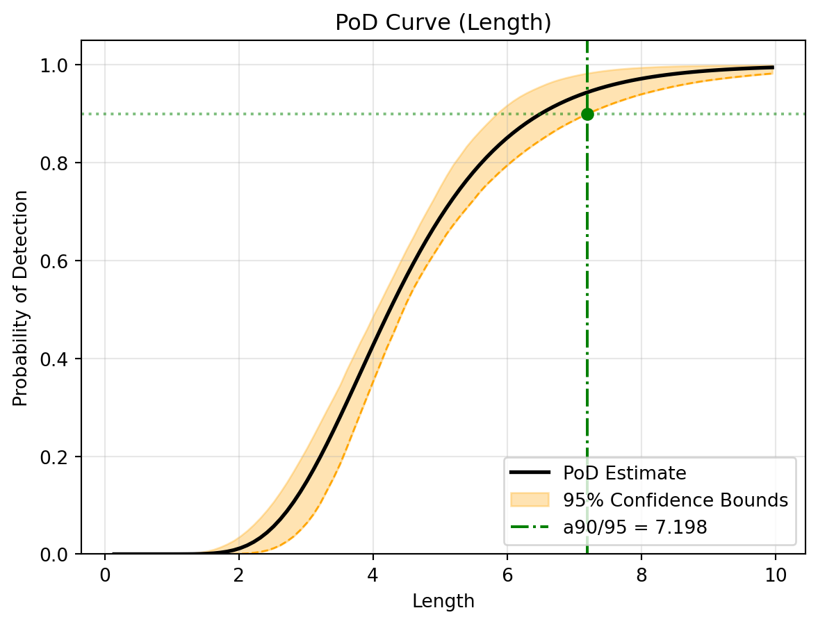
   -> Classical a90/95 Reliability Index: 7.198 mm
--- Linear Analysis Complete ---

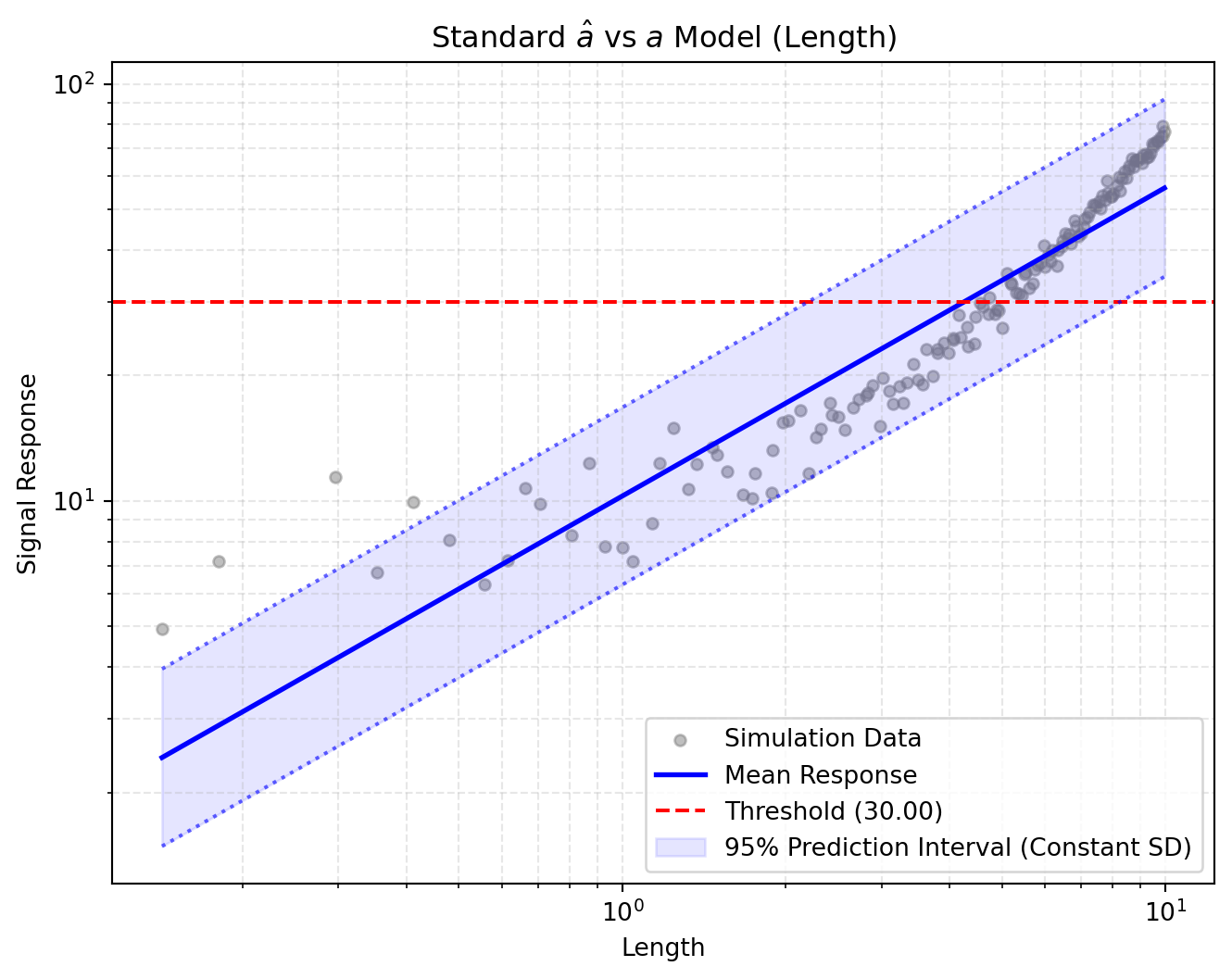
(a) Linear Signal Response Model (Assuming Constant Variance)

(b) Classical PoD Curve (With Bootstrapped Confidence Bounds)

Figure 1: Classical Linear Analysis Results

Tip

Pay attention to the 95% Prediction Interval in the generated plot. Because the classical method assumes constant variance, the bounds are uniformly wide across the entire axis, completely missing the fact that smaller flaws have much tighter signal responses in our dataset!

3. The Generalised Approach (Relaxed)

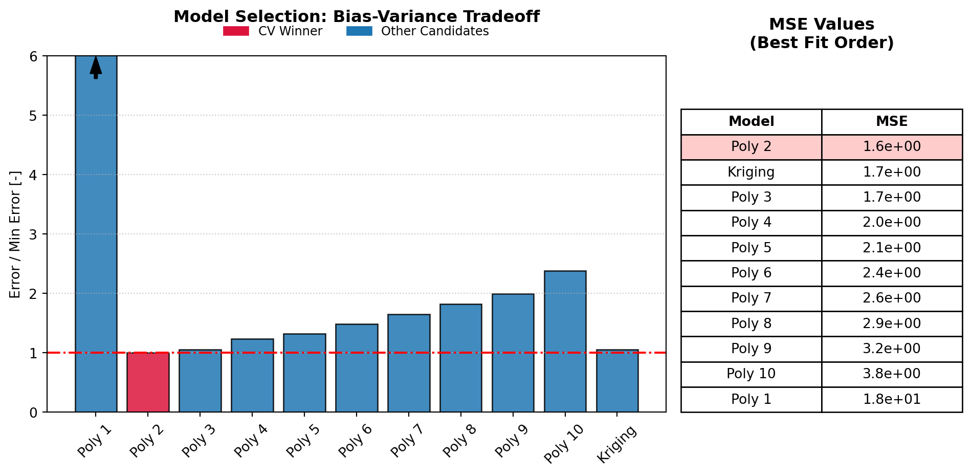
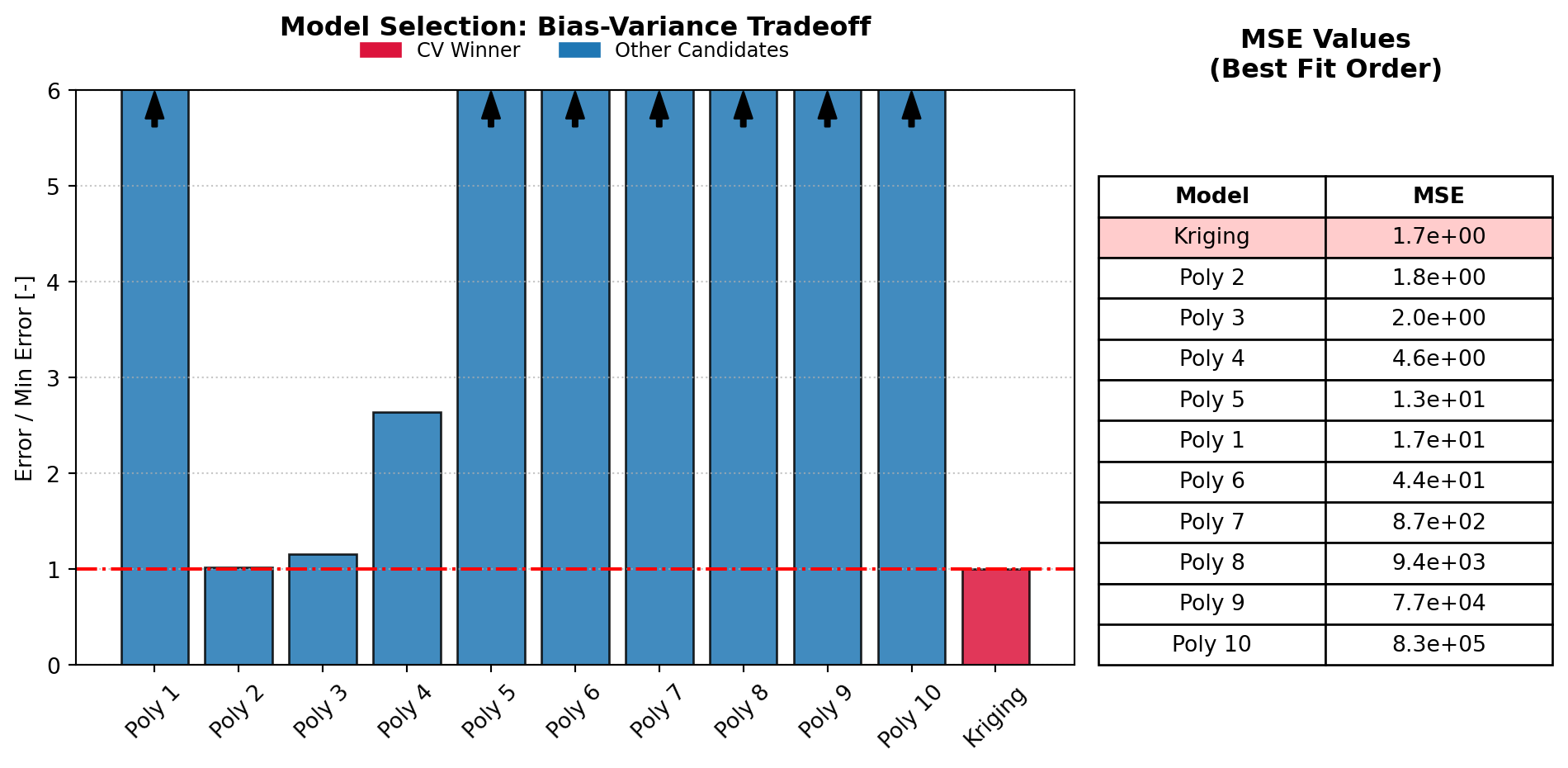
Now, we will run the generalised method. This approach uses cross-validation to select the best non-linear model (Polynomial or Kriging) and automatically models the changing variance using kernel smoothing.

# Run the generalised PoD analysis
# n_jobs=-1 runs the bootstrap process on all available CPU cores
study.pod(
    poi_col="Length", nuisance_col=["Angle", "Roughness"], threshold=30.0, n_jobs=-1
)

# Visualise the relaxed signal fit and PoD curve
study.visualise(show=True)

[Parallel(n_jobs=11)]: Using backend MultiprocessingBackend with 11 concurrent workers.
[Parallel(n_jobs=11)]: Done  19 tasks      | elapsed:   11.2s
[Parallel(n_jobs=11)]: Done 140 tasks      | elapsed:   13.7s
[Parallel(n_jobs=11)]: Done 343 tasks      | elapsed:   17.9s
[Parallel(n_jobs=11)]: Done 626 tasks      | elapsed:   24.1s
[Parallel(n_jobs=11)]: Done 1000 out of 1000 | elapsed:   32.3s finished

--- Starting Reliability Analysis (PoIs: ['Length'] - Nuisance: ['Angle', 'Roughness']) ---
1. Training all surrogate models (Cache Miss)...
-> Selected Model: Kriging (Gaussian Process)
2. Fitting Variance Model & Inferring Distribution (Cache Miss)...
   -> Optimizing bandwidth via LOO-CV...
-> Calculating Total-Order Sobol Indices...
   -> Smoothing Bandwidth: 7.0708
   -> Selected Distribution: norm
3. Integrating PoD Curve from Scratch (Cache Miss)...
4. Running Bootstrap (1000 iterations on 11 cores)...

   -> a90/95 Reliability Index: 5.272
--- Analysis Complete ---

(a) Model Selection (Bias-Variance Tradeoff)

(b) Signal Response Model (Capturing Heteroscedastic Noise)

(c) Generalised PoD Curve (With Bootstrapped Confidence Bounds)

Figure 2: Generalised Relaxed Analysis Results

4. Custom Comparison: Head-to-Head

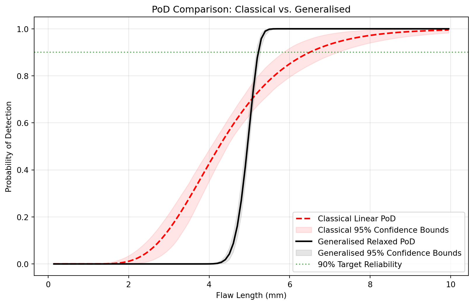
To truly understand the impact of these methodological differences, let’s extract the calculated PoD curves from the SimulationStudy internal state and plot them directly over one another.

# 1. Extract the evaluation grids (X) and PoD curves (Y) from the internal class state
X_linear = study.linear_pod_results["X_eval"]
pod_linear = study.linear_pod_results["curves"]["pod"]
ci_lower_linear = study.linear_pod_results["curves"]["ci_lower"]
ci_upper_linear = study.linear_pod_results["curves"]["ci_upper"]

X_relaxed = study.pod_results["X_eval"].flatten()
pod_relaxed = study.pod_results["curves"]["pod"]
ci_lower_relaxed = study.pod_results["curves"]["ci_lower"]
ci_upper_relaxed = study.pod_results["curves"]["ci_upper"]

# Set up the comparison plot
fig, ax = plt.subplots(figsize=(10, 6))

# 2. Plot Classical Linear Method
ax.plot(
    X_linear,
    pod_linear,
    color="red",
    linestyle="--",
    linewidth=2,
    label="Classical Linear PoD",
)
# Shade Classical Bounds instead of plotting a single line
ax.fill_between(
    X_linear,
    ci_lower_linear,
    ci_upper_linear,
    color="red",
    alpha=0.1,  # Keep alpha low so we can see overlaps
    label="Classical 95% Confidence Bounds",
)

# 3. Plot Generalised Relaxed Method
ax.plot(
    X_relaxed, pod_relaxed, color="black", linewidth=2, label="Generalised Relaxed PoD"
)
# Shade Generalised Bounds between lower and upper
ax.fill_between(
    X_relaxed,
    ci_lower_relaxed,
    ci_upper_relaxed,
    color="gray",
    alpha=0.2,
    label="Generalised 95% Confidence Bounds",
)

# Formatting
ax.axhline(
    0.90, color="green", linestyle=":", alpha=0.6, label="90% Target Reliability"
)
ax.set_ylim(-0.05, 1.05)
ax.set_xlabel("Flaw Length (mm)")
ax.set_ylabel("Probability of Detection")
ax.set_title("PoD Comparison: Classical vs. Generalised")
ax.legend(loc="lower right")
ax.grid(True, alpha=0.3)

plt.show()

# Print a comparative summary
print("--- Reliability Summary ---")
print("Target Threshold: 15")

# Find the a90 points (where the LOWER bounds cross 0.90)
try:
    a90_linear = X_linear[np.argmax(ci_lower_linear >= 0.90)]
    a90_relaxed = X_relaxed[np.argmax(ci_lower_relaxed >= 0.90)]

    print(f"Classical a90/95 (Estimated):  {a90_linear:.2f} mm")
    print(f"Generalised a90/95 (Estimated): {a90_relaxed:.2f} mm")

    diff = abs(a90_relaxed - a90_linear)
    print(f"\nDifference in critical sizing: {diff:.2f} mm")
except IndexError:
    print("Curves did not reach 90% reliability.")

Figure 3: Head-to-Head Reliability Comparison

--- Reliability Summary ---
Target Threshold: 15
Classical a90/95 (Estimated):  7.28 mm
Generalised a90/95 (Estimated): 5.30 mm

Difference in critical sizing: 1.98 mm